Algorithmic trading: triple barrier labelling
Table of Contents
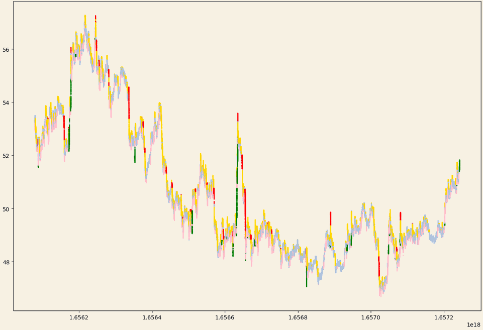
Figure 1: Triple barrier labelling visualisation
Introduction
Triple barrier labelling is a technique for assigning labels to an otherwise unlabelled financial time series, according to some risk parameters. The algorithm sets three barriers: a profit-taking barrier, a stop loss barrier, and a maximum holding period. The labels are assigned based on which barrier is hit first.
The labelled time series is not useful by itself. It is only useful when paired with other inputs or independent variables. This provides a mapping from the inputs to a fixed set of labels, which can then be used to fit a classifier such as a logistic regression model.
Triple barrier labelling and meta labelling
Triple barrier labelling was first introduced in Marcos Lopez de Prado's 2018 book: Advances in Financial Machine Learning 1.
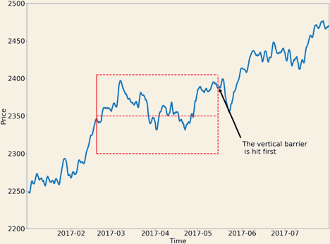
Figure 2: The three barriers visualised
The algorithm uses three barriers to assign class labels to a financial time series. This is useful because, generally speaking, quantitative traders seek to build classifier models and not regression models.
Triple barrier labelling is an improvement over a more primitive approach: the fixed-time horizon method i.e. where observations are labelled based on some fixed distance into the future. The main limitation of this method is that it does not account for market volatility in between the opening and the closing of a position.
In other words, the expected returns of every observation are treated equally regardless of the associated risk. 2
Another problem quantitative traders face is that of position sizing: once we have a model for predicting when to place a bet, we need another model to predict how much capital to place on the bet.
I call this problem meta-labeling because we want to build a secondary ML model that learns how to use a primary exogenous model. 2
Some approaches include:
- Probabilities: when using e.g. a logistic regression, we could use the class probability to size a position, such that a higher probability = larger bet size.
- Conformal prediction: an improvement over raw probabilities - a prediction's conformity measure can be used to size a position, such that higher conformity = larger bet size.
- Kelly criterion: the optimum bet size formula can be used in conjunction with either of the two previous methods.
Python implementation
My implementation of the triple barrier algorithm works by consuming price events from a Python iterator or generator object. For each event, a new "potential position" is created and added to a queue. Each subsequent event is checked against all positions in the queue to determine which boundary has been reached. Hence the algorithm's time complexity is theoretically \(O(n^2)\).
The algorithm becomes more computationally expensive (in both space and time) for larger timeouts, since more events need to be stored in the queue structure.
One of the following four labels is assigned to each potential position:
- Long take profit: if the position were a long then the take profit level would have been reached.
- Long stop loss: if the position were a long then the stop loss level would have been reached.
- Short take profit: if the position were a short then the take profit level would have been reached.
- Short stop loss: if the position were a short then the stop loss level would be been reached.
- Timeout: the maximum time a position can be open was reached.
The following diagram illustrates how the algorithm assigns labels:
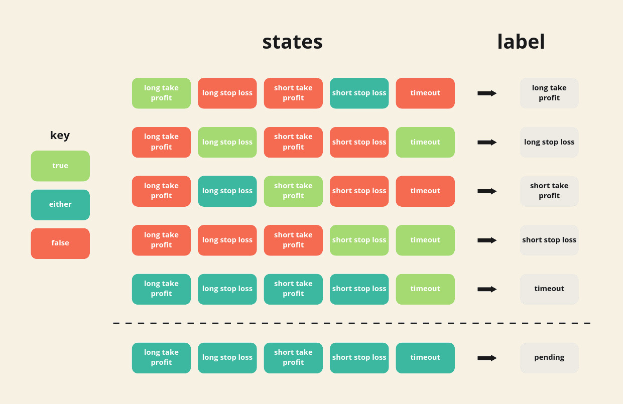
Figure 3: Algorithm state machine diagram
Note: all timestamps are unix with nanosecond granularity.
To begin with, a potential position's states are initialised to "either". Then, as new events come in, the states are updated according to which of the three barriers were hit. When a position's states match one of the combinations above the dashed line, the corresponding label is assigned and the position is removed from the queue.
The algorithm is implemented as a class named TripleBarrier. The
constructor requires a risk parameters object and an iterator that
returns observation objects.
def __init__(self, risk_params, observations):
  self._risk_params = risk_params
  self._observations = observations
  self._observations_generator = None
  self._position_queue = None
When iterating over an instance of TripleBarrier, the object's
observation generator and position queues are initialised:
def __iter__(self):
  # initialise the observations genereator
  self._observations_generator = iter(self._observations)

  # queue for open positions
  self._position_queue = PositionQueue()

  return self
The following method implements the classification logic:
@staticmethod
def assign_label(states):
  # expand the states vector
  long_tp, long_sl, short_tp, short_sl, to = states

  # classify
  if long_tp and not (long_sl or short_tp or to):
    return "long_take_profit"
  elif long_sl and to and not (long_tp or short_tp or short_sl):
    return "long_stop_loss"
  elif short_tp and not (long_tp or short_sl or to):
    return "short_take_profit"
  elif short_sl and to and not (long_tp or long_sl or short_tp):
    return "short_stop_loss"
  elif to:
    return "timeout"
  else:
    return "pending"
In each iteration, all open position are checked - to see if they have
a label other than "pending". Until the observations generator raises
StopIteration, the algorithm will consume observations and add them
to the position queue:
def __next__(self):
  # observations that were labelled in this iteration
  labelled = []

  # observe next event
  obs = next(self._observations_generator)

  # get boundaries for the new position
  long_boundaries, short_boundaries, max_time_ns = \
    self._risk_params.get_boundaries(obs)

  # create the new potential position
  next_pos = \
    Position(obs, long_boundaries, short_boundaries, max_time_ns)

  # add latest observation to previous positions
  for pos in self._position_queue.items():
    pos.add_observation(obs)

  # check if any previous positions can be labelled
  for pos in self._position_queue.items():
    states = pos.state_vector()
    label = self.assign_label(states)

    if label == "pending":
        # no need to check further because we assume they are
        # ordered by timestamp
        break
    else:
        # the position has been labelled
        labelled.append(Labelled(pos, label))
        self._position_queue.remove(pos)

  # push new position to the position queue
  self._position_queue.append(next_pos)

  # return iteration metadata
  return LabellerIteration(
    unix_ts_ns=obs.unix_ts_ns(),
    price=obs.price(),
    backlog_count=len(self._position_queue),
    labelled=labelled)
The output of each iteration is an instance of LabellerIteration,
which wraps some metadata about the labeller object's current state,
as well as any observations that were successfully labelled in that
iteration.
It is up to the user of this class to collect all of the labels into whatever data structure suits them. For example, one might aggregate all labels into a Pyspark RDD.
Demonstration
The chart at the top of this post illustrates the output of the triple barrier algorithm with colours assigned to each label:
- Red: Short stop loss hit.
- Green: Long take profit hit.
- Yellow: Short stop loss hit.
- Pink: Long stop loss hit.
- Grey: max time exceeded.
Figure 4: Triple barrier labelling visualisation
The risk parameters, which are the same in both directions, are as follows:
- Take profit: 1.5%.
- Stop loss: 0.5%.
- Timeout: 15 minutes.
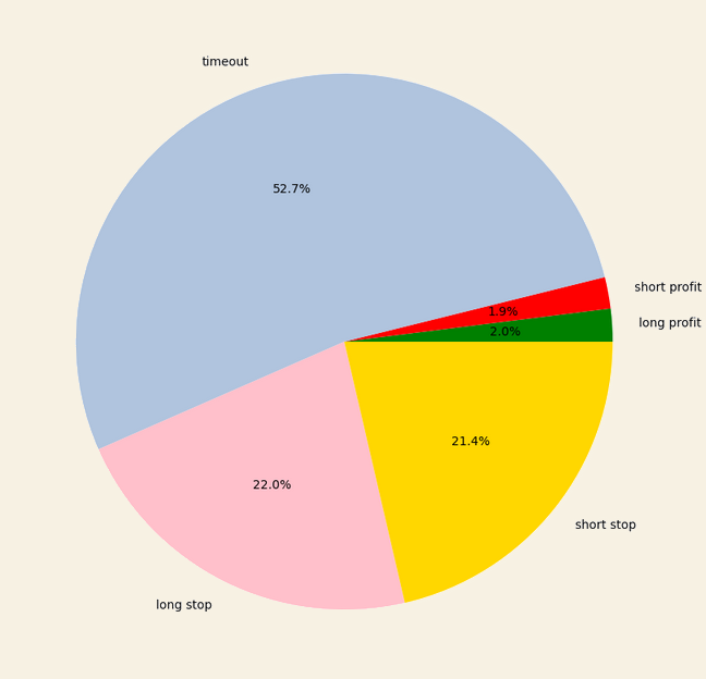
Figure 5: Label count pie chart
As you can see, most of the time the market's behaviour is not within our risk parameters. In other words, only 4% of price movements were profitable and were not stopped-out. This is expected behaviour because most of the time the market is not sufficiently volatile.